| |
|
|
r2 - 09 Jan 2016 - 09:44 - DenisDerkach |
|
r1 - 21 Jul 2015 - 08:10 - DenisDerkach |
|
|---|
| |
| |
|
New Physics Fit results: Winter 2016 |
|
New Physics Fit results: Summer 2015 |
|
|
|
The fit presented here is meant to constrain the NP contributions to |? F|=2 transitions by using the available experimental information on loop-mediated processes In general, NP models introduce a large number of new parameters: flavour changing couplings, short distance coefficients and matrix elements of new local operators. The specific list and the actual values of these parameters can only be determined within a given model. Nevertheless mixing processes are described by a single amplitude and can be parameterized, without loss of generality, in terms of two parameters, which quantify the difference of the complex amplitude with respect to the SM one. Thus, for instance, in the case of  mixing we define mixing we define |
|
The fit presented here is meant to constrain the NP contributions to |? F|=2 transitions by using the available experimental information on loop-mediated processes In general, NP models introduce a large number of new parameters: flavour changing couplings, short distance coefficients and matrix elements of new local operators. The specific list and the actual values of these parameters can only be determined within a given model. Nevertheless mixing processes are described by a single amplitude and can be parameterized, without loss of generality, in terms of two parameters, which quantify the difference of the complex amplitude with respect to the SM one. Thus, for instance, in the case of mixing we define |
|
|
|
 |
|
|
|
|
|
where  includes only the SM box diagrams, while includes only the SM box diagrams, while  also includes the NP contributions. In the absence of NP effects, also includes the NP contributions. In the absence of NP effects,  and and  by definition. In a similar way, one can write by definition. In a similar way, one can write |
|
where includes only the SM box diagrams, while also includes the NP contributions. In the absence of NP effects, and by definition. In a similar way, one can write |
|
|
|
![C_{\epsilon_K} = \frac{\mathrm{Im}[\langle
K^0|H_{\mathrm{eff}}^{\mathrm{full}}|\bar{K}^0\rangle]}
{\mathrm{Im}[\langle
K^0|H_{\mathrm{eff}}^{\mathrm{SM}}|\bar{K}^0\rangle]}\,,\qquad
C_{\Delta m_K} = \frac{\mathrm{Re}[\langle
K^0|H_{\mathrm{eff}}^{\mathrm{full}}|\bar{K}^0\rangle]}
{\mathrm{Re}[\langle
K^0|H_{\mathrm{eff}}^{\mathrm{SM}}|\bar{K}^0\rangle]}\,.
\label{eq:ceps}](/foswiki/pub/UTfit/ResultsWinter2016NP/_MathModePlugin_67ab6a9a7b559aa5224ab6e8d6c0ecab.png) |
|
|
|
|
|
Concerning  , to be conservative, we add to the short-distance contribution a possible long-distance one that varies with a uniform distribution between zero and the experimental value of . , to be conservative, we add to the short-distance contribution a possible long-distance one that varies with a uniform distribution between zero and the experimental value of . |
|
Concerning , to be conservative, we add to the short-distance contribution a possible long-distance one that varies with a uniform distribution between zero and the experimental value of . |
|
|
|
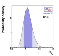
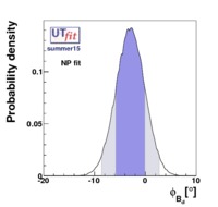
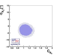
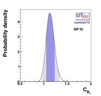
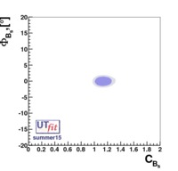
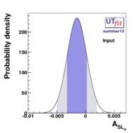
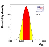
The experimental quantities determined from the mixings are related to their SM counterparts and the NP parameters by the following relations: |
|
The experimental quantities determined from the mixings are related to their SM counterparts and the NP parameters by the following relations: |
|
|
|
 |
|
|
|
|
|
in a self-explanatory notation. |
|
in a self-explanatory notation. |
|
|
|
All the measured observables can be written as a function of these NP parameters and the SM ones ? and ?, and additional parameters such as masses, form factors, and decay constants. |
|
All the measured observables can be written as a function of these NP parameters and the SM ones ? and ?, and additional parameters such as masses, form factors, and decay constants. |
|
| |
|
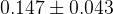
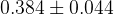
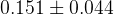
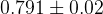
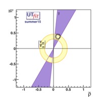
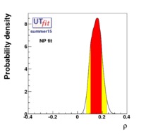
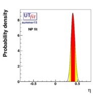
CKM matrix thus looks like 
|
|
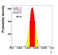
The fit results for all the nine CKM elements are 
|
|
| |
|
|
r2 - 09 Jan 2016 - 09:44 - DenisDerkach |
|
r1 - 21 Jul 2015 - 08:10 - DenisDerkach |
|
|---|
| |


![\alpha [^{\circ}]](/foswiki/pub/UTfit/ResultsWinter2016NP/_MathModePlugin_7f9d77ff9ef45eb8303abd2177efaa0d.png)

![\beta [^{\circ}]](/foswiki/pub/UTfit/ResultsWinter2016NP/_MathModePlugin_d29a2254c73881a349faf62902020dd2.png)

![\gamma [^{\circ}]](/foswiki/pub/UTfit/ResultsWinter2016NP/_MathModePlugin_d441395f3c6b5d6d14b98a13ae4b8837.png)


![\phi_{B_{d}} [^{\circ}]](/foswiki/pub/UTfit/ResultsWinter2016NP/_MathModePlugin_e7bdbf0a9f051522c1f90b3639728013.png)


![\phi_{B_{s}} [^{\circ}]](/foswiki/pub/UTfit/ResultsWinter2016NP/_MathModePlugin_8e3e52e8fa1dc4be050940fb4dc3291a.png)


![\,\alpha [^{\circ}]](/foswiki/pub/UTfit/ResultsWinter2016NP/_MathModePlugin_e05c751c79f7a7933981b51edd7759fb.png)

![\,\beta [^{\circ}]](/foswiki/pub/UTfit/ResultsWinter2016NP/_MathModePlugin_32b6b8a2c9036a9cb59f5fc29194388e.png)

![\,\gamma [^{\circ}]](/foswiki/pub/UTfit/ResultsWinter2016NP/_MathModePlugin_346b4369d40fd8964bda0f769a5b4bbe.png)


![\,\phi_{B_{d}} [^{\circ}]](/foswiki/pub/UTfit/ResultsWinter2016NP/_MathModePlugin_0099383160d64332d39305e02dac12bc.png)


![\,\phi_{B_{s}} [^{\circ}]](/foswiki/pub/UTfit/ResultsWinter2016NP/_MathModePlugin_ff01b905362e6cc6c4067ca2dd53b0bc.png)