- Home
- Constraints
- Fit Results
- Historical Plots
- Papers and Conferences
- CKM Formalism
- Statistical Method
- Contacts
- Feedback
Gamma Combination from the UTfit goup


We use the relevant post-ICHEP 2012 HFAG averages as inputs.
The results of combination:
The predictions of the observables coming from the full fit:
| Parameter | Full fit |
|---|---|
![\gamma [^{\circ}]](/foswiki/pub/UTfit/GammaFromTrees/_MathModePlugin_d441395f3c6b5d6d14b98a13ae4b8837.png) |
 |
![\delta_{B}(DK) [^{\circ}]](/foswiki/pub/UTfit/GammaFromTrees/_MathModePlugin_41e661b01cefdd9ec2084738b64160f3.png) |
 |
 |
 |
![\delta_{B}(DK^{*}) [^{\circ}]](/foswiki/pub/UTfit/GammaFromTrees/_MathModePlugin_1baa48393b03b96f22571066583a25b8.png) |
 |
 |
 |
![\delta_{B}(D^{*}K) [^{\circ}]](/foswiki/pub/UTfit/GammaFromTrees/_MathModePlugin_5211b61dcb830d9a98ee9a7878d74aff.png) |
 |
 |
 |
![\delta_{B0}(DK^{0}) [^{\circ}]](/foswiki/pub/UTfit/GammaFromTrees/_MathModePlugin_060131b4fd1a7430d5cc8dca6c37fdf8.png) |
 |
 |
 |
|
![\,\gamma [^{\circ}]](/foswiki/pub/UTfit/GammaFromTrees/_MathModePlugin_346b4369d40fd8964bda0f769a5b4bbe.png)

|
![\,\delta_{B}(DK) [^{\circ}]](/foswiki/pub/UTfit/GammaFromTrees/_MathModePlugin_de1251af0a072fb83f6dd951669769db.png)

|


|
![\,\delta_{B}(DK^{*}) [^{\circ}]](/foswiki/pub/UTfit/GammaFromTrees/_MathModePlugin_5164e268a514bb26250f2bad6b8038e2.png)

|


|
![\,\delta_{B}(D^{*}K) [^{\circ}]](/foswiki/pub/UTfit/GammaFromTrees/_MathModePlugin_59f1351d3c4dd771bf1d0e886a13457a.png)

|


|
![\,\delta_{B0}(DK^{0}) [^{\circ}]](/foswiki/pub/UTfit/GammaFromTrees/_MathModePlugin_5e88e4e05fc48c6d86a012b46b14cf1b.png)

|

| Parameter | Full fit |
|---|---|
 |
 |
 |
 |
 |
 |
 |
 |
 |
 |
 |
 |
 |
 |
 |
 |
 |
 |
 |
 |
 |
 |
 |
 |
 |
 |
 |
 |
 |
 |
 |
 |
 |
 |
 |
 |
 |
 |
 |
 |
 |
 |
 |
 |
 |
 |
 |
 |
 |
 |
 |
 |
 |
 |
 |
 |
 |
 |
 |
 |
 |
 |
 |
 |
The angle  of the CKM triangle can be measured comparing
  and
and  mediated transitions in
  decays. The decays proceed through the following diagrams:

These diagrams are practically free from the New Physics contribution.
There are three methods to extract relevant information, each of them deals with its own  decay:
 and the relative
  conserving phase
 between the two amplitudes. These parameters depend on the
  decay under investigation.
of the CKM triangle can be measured comparing and mediated transitions in decays. The decays proceed through the following diagrams:
decay:
- a singly Cabibbo-suppressed CP eigenstate, like
 for Gronau-London-Wyler (GLW) method;
- a doubly Cabibbo-suppressed flavor eigenstate, like
 for Atwood-Dunietz-Soni (ADS) method;
- a Cabibbo-allowed self-conjugate 3-body state, like
 for Giri-Grossman-Soffer-Zupan (GGSZ) method.
and the relative conserving phase between the two amplitudes. These parameters depend on the decay under investigation.
The Gronau-London-Wyler (GLW) method (M. Gronau, D. Wyler, Phys. Rev. Lett. B {\bf 253} (1991) 483; M. Gronau, D. London, Phys. Rev. Lett. B {\bf 265} (1991) 172) is based on the reconstruction of the decay to  , where and
  decay
to -even or -odd eigenstates. The
decay
to -even or -odd eigenstates. The  modes normally used are:
 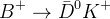 , with
  is also reconstructed.
The four observables for this method are formed in the following
way:
is also reconstructed.
The four observables for this method are formed in the following
way:

 This set can provide an information on , , and
  with an 8-fold ambiguity for the phases.
decay to , where and decay
to -even or -odd eigenstates. The modes normally used are: -
 :
:  ,
,  ;
;
-
 :
:  ,
,  ,
,  ,
,  , and
, and  .
.
, with is also reconstructed.
The four observables for this method are formed in the following
way:
This set can provide an information on , , and with an 8-fold ambiguity for the phases.
In the ADS method (I. Dunietz, Phys. Rev. Lett. B 270 (1991) 75; Phys. Rev. Lett. D 52 (1995) 3048; D. Atwood, I. Dunietz and A. Soni, Phys. Rev. Lett. 78, 3257 (1997)), is measured from the study of  decays, where mesons decay into non eigenstate final states. The suppression of
  transition with respect to the
  one is partly overcome by the study of decays of the meson in final states which can proceed in two ways: either through a favored decay followed by a doubly-Cabibbo-suppressed decay, or through a suppressed
  decay followed by a Cabibbo-favored decay.
Neglecting -mixing effects, which in the SM give very small corrections to \g\ and do not affect the measurement, the measured ratios
decay followed by a Cabibbo-favored decay.
Neglecting -mixing effects, which in the SM give very small corrections to \g\ and do not affect the measurement, the measured ratios  and
and  are related to the and mesons' decay parameters through the following relations:
![R_{\rm ADS}=\frac{\Gamma(B^{+}\rightarrow [\bar f]_{D^{0}} K^{+})+\Gamma(B^{-}\rightarrow [f]_{D^{0}} K^{-})}{\Gamma(B^{+}\to[f]_{D^{0}} K^{+})+\Gamma(B^{-}\to[\bar f]_{D^{0}} K^{-})}=(r_{B}^2+r_{D}^2+2 r_{B} r_{D} k_{D}k_{B}\cos\gamma\cos\delta),](/foswiki/pub/UTfit/GammaFromTrees/_MathModePlugin_6f88dbde825ec879a69f94b702543683.png)
![A_{\rm ADS}=\frac{\Gamma(B^{+}\rightarrow [\bar f]_{D^{0}} K^{+})-\Gamma(B^{-}\rightarrow [f]_{D^{0}} K^{-})}{\Gamma(B^{+}\to[f]_{D^{0}} K^{+})+\Gamma(B^{-}\to[\bar f]_{D^{0}} K^{-})}=(r_{B}^2+r_{D}^2+2 r_{B} r_{D} k_{D}k_{B}\sin\gamma\sin\delta)/R_{\rm ADS},](/foswiki/pub/UTfit/GammaFromTrees/_MathModePlugin_9c76bf82e9d7630117d2ae806cedd7c4.png) with:
with:
 In case of the
  analysis with
  we use the following ratios:
![R^{\pm}=\frac{\Gamma(B^{\pm}\rightarrow [\bar f]_{D^{0}} K^{\pm})}{\Gamma(B^{\pm}\to[f]_{D^{0}} K^{\pm})}=(r_{B}^2+r_{D}^2+2 r_{B} r_{D} k_{D}k_{B}\cos(\gamma\pm\delta)),](/foswiki/pub/UTfit/GammaFromTrees/_MathModePlugin_41afc139cc9ed5b97c8bcc7e836d6ea5.png) The used observables are connected to the "classical"
The used observables are connected to the "classical"  and
and  set by simple relations:
  and
and  .
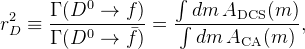
The values of
.
The values of  and
and  are taken from our study of charm mixing or the CLEO-c collaboration results. The ratio
  has been
measured in different experiments and we take the average value from PDG.
has been
measured in different experiments and we take the average value from PDG.
is measured from the study of decays, where mesons decay into non eigenstate final states. The suppression of transition with respect to the one is partly overcome by the study of decays of the meson in final states which can proceed in two ways: either through a favored decay followed by a doubly-Cabibbo-suppressed decay, or through a suppressed decay followed by a Cabibbo-favored decay.
Neglecting -mixing effects, which in the SM give very small corrections to \g\ and do not affect the measurement, the measured ratios and are related to the and mesons' decay parameters through the following relations:
with:
In case of the analysis with we use the following ratios:
The used observables are connected to the "classical" and set by simple relations: and .
The values of and are taken from our study of charm mixing or the CLEO-c collaboration results. The ratio has been
measured in different experiments and we take the average value from PDG.
The Giri Grossman Soffer Zupan (GGSZ), also called Dalitz method (A. Giri, Y. Grossman, A. Soffer and J. Zupan, Phys. Rev. D 68, 054018 (2003)) is based on the reconstruction of the decay to , where and decay  ;
The four observables for this method are formed in the following way:
;
The four observables for this method are formed in the following way:

decay to , where and decay ;
The four observables for this method are formed in the following way:
Powered by
 Ideas, requests, problems regarding this web site? Send feedback