- Home
- Constraints
- Fit Results
- Historical Plots
- Papers and Conferences
- CKM Formalism
- Statistical Method
- Contacts
- Feedback


In this page we present the results obtained for a set of interesting UT parameters in the framework of the Standard Model an some New Physics Models using all the available experimental and theoretical inputs which are available.
Inputs to this analysis consist of a large body of both experimental measurements and theoretically determined parameters.
All the analyses presented here rely on the several measurements: |Vub| / |Vcb|, Dmd, Dms, and the measurements of CP-violating quantities
in the kaon (εK) and in the B sectors with the measurements of α (using ππ, ρρ and πρ modes), γ (using D()K() modes), 2β + γ (using D(*)π(ρ)
modes), and sin2β and cos 2β from B0 → J/ψKS and B0 → J/ψK* respectively. Among the theoretical parameter, LQCD calculations play a central role
The results are presented in a summary table and in a series of probability density functions. The tables contain three entries per variable : the input ("direct") value, the output value and the prediction ("indirect determination") for this variable in a given model.
The indirect determination of a particular quantity obtained performing the Unitarity Triangle fit in a given Model, including all the available constraints except from the direct measurement of the parameter of interest, gives a prediction of the quantity based on formulas which are valid in that given Model. The interest of this procedure is to quantify the agreement of all the measured quantities by the comparison between indirect parameter determinations and their direct experimental/theortical determinations. Let's consider for example the Standard Model. The comparison between these predictions and a direct measurements can thus quantify the agreement of the single measurement with the overall fit and possibly reveal new physics phenomena.
For some of the quantity we present the so called compatibility plots. In Unitarity Triangle fits based on a χ2 minimization, a conventional evaluation of compatibility stems automatically from the value of the χ2 at its minimum. The compatibility between constraints in the Bayesian approach is simply done by comparing two different p.d.f.’s.
Let us consider, for instance, two p.d.f.’s for a given quantity obtained from the Unitarity Triangle fit, f(x1), and from a direct measurement, f(x2): their compatibility is evaluated by constructing the p.d.f. of the difference variable, x2 − x1, and by estimating the distance of the most probable value from zero in units of standard deviations. The latter is done by integrating this p.d.f. between zero and the most probable value and converting it into the equivalent number of standard deviations for a Gaussian distribution 1. The advantage of this approach is that no approximation is made on the shape of p.d.f.’s. In the following analysis, f(x1) is the p.d.f. predicted by the Unitarity Triangle fit while the p.d.f of the measured quantity, f(x2), is taken Gaussian for simplicity. The number of standard deviations between the measured value, ¯x2 ± σ(x2), and the predicted value (distributed according to f(x1)) is plotted as a function of ¯x2 (x-axis) and σ(x2) (y-axis). The compatibility between x1 and x2 can be then directly estimated on the plot, for any central value and error of the measurement of x2.
The color code indicates the compatibility between direct and indirect determinations, given in terms of standard deviations, as a function of the measured value and its experimental uncertainty. The crosses indicate the direct world average measurement values.
| Parameter | Input value | Full fit | SM Prediction |
|---|---|---|---|
 |
 |
 |
|
 |
|
 |
|
 |
|
 |
|
 |
|
 |
|
 |
|
 |
|
 |
 |
 |
|
 |
 |
 |
 |
 |
 |
 |
 |
 |
|
|
|
 |
|
|
|
 |
|
|
|
 |
|
 |
|
 |
 |
|
|
 |
 |
|
|
 |
 |
|
 |
 |
 |
|
 |
 |
 |
|
|
 |
 |
|
|
 |
 |
 |
 |
 |
 |
 |
 |
 |
 |
 |
 |
 |
 |
 |
 |
![\alpha, [^{\circ}]](/foswiki/pub/UTfit/Results/_MathModePlugin_fd9cffa79bba1cefe698ffb780948bfd.png) |
 |
 |
 |
![\beta, [^{\circ}]](/foswiki/pub/UTfit/Results/_MathModePlugin_681db302c08739ecb70979d0c2f99469.png) |
|
 |
 |
 |
 |
 |
 |
 |
 |
 |
 |
![2\beta+\gamma, [^{\circ}]](/foswiki/pub/UTfit/Results/_MathModePlugin_0afe674b922eb68c67432526ab5f530d.png) |
 |
 |
 |
![\gamma, [^{\circ}]](/foswiki/pub/UTfit/Results/_MathModePlugin_c377dff471191b5a2ce708a386f857ea.png) |
 |
 |
 |
 |
 |
 |
 |
 |
 |
 |
 |
 |
|
 |
|

|
|
|


|
|


|


|
|


|
|
|
|


|
|
|
|


|


|


|


|


|
|
|
|


|
|
|
|


|
|
|
|


|
|
|
|


|
|
|
|


|
|
|
|


|
|
|
|
![\,\alpha, [^{\circ}]](/foswiki/pub/UTfit/Results/_MathModePlugin_ae362e71d38e928a75dcc639252277fa.png)


|
|
![\,\beta, [^{\circ}]](/foswiki/pub/UTfit/Results/_MathModePlugin_e51236bcc048af447e95d21eef282e8c.png)


|
|
|
|


|
|
|
|


|
|
|
|
![\,2\beta+\gamma, [^{\circ}]](/foswiki/pub/UTfit/Results/_MathModePlugin_079308c321dda6eaa70aab72a9dc96e3.png)


|
|
|
|
![\,\gamma, [^{\circ}]](/foswiki/pub/UTfit/Results/_MathModePlugin_724ac13299d2e41ce3b151d52dc1545f.png)


|
|
|
|


|
|
|
|


|

| Constraints, Parameters | Value | Gaussian Error | Flat Error | Comments |
|---|---|---|---|---|
| |
 |
 |
- | - |
![\left | V_{cb} \right |~[10^{-3}]](/foswiki/pub/UTfit/Results/_MathModePlugin_fc4661c2241d0f10c4a25aff9ae90e4e.png) |
 |
 |
- | Average of exclusive |
| |
 |
 |
- | Average of inclusive |
![\left | V_{ub} \right |~[10^{-4}] \mathrm{(excl.)}](/foswiki/pub/UTfit/Results/_MathModePlugin_b2cc05b80c5a18e3f97b1d3243c75007.png) |
 |
 |
- | HFAG BR + Lattice QCD |
![\left | V_{ub} \right |~[10^{-4}] \mathrm{(incl.)}](/foswiki/pub/UTfit/Results/_MathModePlugin_38236d194dff1b2117145d3b723f39bc.png) |
 |
 |
|
HFAG average |
 |
 |
 |
- | - |
 |
 |
 |
- | - |
![\Delta m_d~[ps^{-1}]](/foswiki/pub/UTfit/Results/_MathModePlugin_d8d6be4b6a774788c18ee6d0c92506fc.png) |
 |
 |
- | WA (CDF/CLEO/LEP/BaBar/Belle) |
![\Delta m_s~[ps^{-1}]](/foswiki/pub/UTfit/Results/_MathModePlugin_c981187e0dfde242fddf843217eed79c.png) |
 |
 |
- | CDF Likelihood is used |
![m_t~[GeV/c^2]](/foswiki/pub/UTfit/Results/_MathModePlugin_505762405777afe7e25bf6489fff3318.png) |
 |
 |
- | (CDF/D0) |
![f_{B_s}\sqrt{B_{B_s}}~[MeV]](/foswiki/pub/UTfit/Results/_MathModePlugin_3b7dafec0324b2c1acab04fe6ab32f3b.png) |
 |
 |
- | Lattice QCD |
 |
 |
 |
- | Lattice QCD |
![|\varepsilon_K|~[10^{-3}]](/foswiki/pub/UTfit/Results/_MathModePlugin_47592daf0d9fd5e3f983ff40c533890d.png) |
 |
 |
- | - |
 |
 |
 |
- | Lattice QCD |
![f_K~[GeV]](/foswiki/pub/UTfit/Results/_MathModePlugin_c40b338c56ce56f4045de5da182ee6e6.png) |
 |
- | - | - |
![\Delta m_K~[10^{-2}~ps^{-1}]](/foswiki/pub/UTfit/Results/_MathModePlugin_66e84a6499e57d9bb4e87ed386c73c1b.png) |
 |
- | - | - |
![M_{K^0}~[GeV/c^2]](/foswiki/pub/UTfit/Results/_MathModePlugin_d578fd13f3b19013106b949945133917.png) |
 |
- | - | - |
Under construction
In the Unitarity Triangle fits the non perturbative QCD parameters enter in the expressions of several contraints :
 .
Let's consider schematically the dependence of these observable in terms of the non perturbative QCD parameters :
.
Let's consider schematically the dependence of these observable in terms of the non perturbative QCD parameters :
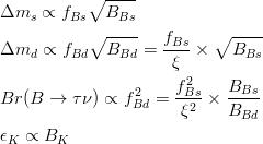 .
We decide to express these observable in terms of five LQCD parameters
.
We decide to express these observable in terms of five LQCD parameters
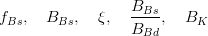
 (exclusive) and
  .
.
.
Let's consider schematically the dependence of these observable in terms of the non perturbative QCD parameters :
.
We decide to express these observable in terms of five LQCD parameters
(exclusive) and .
Powered by
 Ideas, requests, problems regarding this web site? Send feedback